

LSRFormer模块是在“LSRFormer: Efficient Transformer Supply Convolutional Neural Networks with Global Information for Aerial Image Segmentation”这篇论文中提出的,其融合了ViT和CNN的优势,主要解决的是CNN难以建模全局依赖关系和ViT计算成本高且难以保留局部空间细节的问题。
很久之前的LSRFormer论文总结请见以下文章:

前置问题和知识
CNN的问题:由于卷积核大小的限制,使其由感受野范围受限的问题,很难获取图像中远距离像素的关系。
ViT的问题:全局Token交互成本很高(\(O(n^2)\)),不适用于(不是说不能用,而是性能耗费太多)大尺寸的图片,比如1024×1024的LoveDA数据集样本。
Self Attention:自注意力(Self Attention, SA)是通过计算Token与所有其他Token之间的关系来实现全局信息交换的。它使用三个线性变换矩阵(Wq、Wk、Wv)分别获取查询(Q)、键(K)和值(V)。通过点乘计算Q和K得到注意力图(可以体现Token之间的相似性),然后将注意力图与值(V)相乘得到输出结果。这样就能这使得SA具有全局感受野这一特点。
LSRFormer模块
![图片[1] - AI科研 编程 读书笔记 - 【人工智能】对LSRFormer模块的理解——遥感图像语义分割 - AI科研 编程 读书笔记 - 小竹の笔记本](https://img.smallbamboo.cn/i/2025/02/28/67c14d0654b65.png)
![图片[2] - AI科研 编程 读书笔记 - 【人工智能】对LSRFormer模块的理解——遥感图像语义分割 - AI科研 编程 读书笔记 - 小竹の笔记本](https://img.smallbamboo.cn/i/2025/07/05/68688364b6c39.png)
![图片[3] - AI科研 编程 读书笔记 - 【人工智能】对LSRFormer模块的理解——遥感图像语义分割 - AI科研 编程 读书笔记 - 小竹の笔记本](https://img.smallbamboo.cn/i/2025/02/28/67c14d1514ee6.png)
Split Windows
在进入SA之前,输入特征图先被分割为多个窗口。作者在研究中发现窗口尺寸设置为4时最佳,后面的讲解以及作者图中的示例都以窗口尺寸为4为例。
在图3和图4中可以看到,红色的线就是窗口划分边界。
代码中通过window_partition函数实现。当然还有一个反向操作,是将多个窗口合并,是通过window_reverse函数实现的。
def window_partition(x, window_size):
    """
        x: (B, H, W, C) Returns:windows: (num_windows*B, window_size, window_size, C)
    """
    B, H, W, C = x.shape
    x = x.view(B, H // window_size[0], window_size[0], W // window_size[1], window_size[1], C).contiguous()
    windows = x.permute(0, 1, 3, 2, 4, 5).contiguous().view(-1, window_size[0], window_size[1], C).contiguous()
    return windows

def window_reverse(windows, window_size, H, W):
    """
    Args:
        windows: (num_windows*B, window_size, window_size, C)   Returns:x: (B, H, W, C)
    """
    B = int(windows.shape[0] / (H * W / window_size[0] / window_size[1]))
    x = windows.view(B, H // window_size[0], W // window_size[1], window_size[0], window_size[1], -1).contiguous()
    x = x.permute(0, 1, 3, 2, 4, 5).contiguous().view(B, H, W, -1).contiguous()
    return x
LR-SA(长程自注意力)
LR-SA主要是为了先在之前分好的窗口的边缘处建立长距离的依赖关系,用比较低的计算成本(因为边界处的像素远远小于整体的总像素数量)获得近似的全局特征。
如图4所示,是一个8×8的特征图,分窗口(4×4)之后,LR-SA会识别在窗口边缘的Token,也就是图中橙色和黄色的框圈起来的像素,进一步计算它们的矩阵索引。然后用这些索引提取交界处的Token,通过卷积进一步减少Token的数量。之后执行标准的SA,执行后将学习到的Token上采样并恢复到原始尺寸,也就是基于刚刚提到的window_reverse函数。下一步利用之前提取的索引将其添加到原始特征图中(相当于是一个残差连接的变体),为SR-SA做准备。
下面是LR-SA的代码流程部分。
        # input x: b c h w
        # step1:reduce dim of x
        x_reduction = self.conv_reduce(x) # w,h /2 ; c /4
        x_reduction = x_reduction.permute(0,2,3,1).contiguous() # bchw->bhwc

        # add :pad feature maps to multiples of window size 4
        H,W = x_reduction.shape[1],x_reduction.shape[2]
        pad_r = int(((4 - W % 4) % 4)/2)
        pad_b= pad_l = pad_t = pad_r
        if pad_r>0:
            x_reduction = F.pad(x_reduction, (0, 0, pad_l, pad_r, pad_t, pad_b),mode='reflect')

        # get index of window border
        border_index = torch.Tensor(self.get_index(x_reduction.shape[2])).int().to(x_reduction.device)

        # long range attn
        x_h = torch.index_select(x_reduction ,1, border_index).permute(0,3,1,2).contiguous()  # [1, 16, 62, 128]
        x_h = self.h_conv(x_h).permute(0,2,3,1).contiguous()    # b c h w -> b h w c  [1, 31, 64, 16]
        b_,h_,w_,c_ = x_h.shape
        x_h = window_partition(x_h,[1,w_]).view(-1,1*w_,c_).contiguous()    # [31, 64, 16]

        x_w = torch.index_select(x_reduction,2,border_index).permute(0,3,2,1).contiguous()   # [1, 16, 62, 128]
        x_w = self.w_conv(x_w).permute(0,2,3,1).contiguous()    # b c h w -> b h w c  [1, 31, 64, 16]
        x_w = window_partition(x_w,[1,w_]).view(-1,1*w_,c_).contiguous()    # [31, 64, 16]

        x_total = torch.cat([x_h,x_w],dim=0)

        x_h,x_w = torch.chunk(self.global_attn(x_total),2,0)
        x_h,x_w = x_h.contiguous(),x_w.contiguous()
        x_h,x_w = window_reverse(x_h,[1,w_],h_,w_).permute(0,3,1,2).contiguous(),window_reverse(x_w,[1,w_],h_,w_).permute(0,3,2,1).contiguous()
        x_h,x_w = F.interpolate(x_h,scale_factor=2,mode='bilinear', align_corners=True),F.interpolate(x_w, scale_factor=2,mode='bilinear', align_corners=True)
        x_h,x_w = x_h.permute(0,2,3,1).contiguous(),x_w.permute(0,2,3,1).contiguous() # [1, 16, 62, 128] [1, 16, 128, 62]

        x_reduction.index_add_(1,border_index,x_h)
        x_reduction.index_add_(2,border_index,x_w)  # bhwc
        # long range attn end
看起来稍显复杂。第一步是x_reduction = self.conv_reduce(x):对输入特征 x 进行维度和空间尺寸的初步缩减。降低计算成本在self.conv_reduce函数里面是通过nn.Conv2d(dim, dim//self.channel_ratio, 2, 2, 0, groups=dim//8)实现的,它将特征图尺寸减半(2,2,0 表示步长为2,会降采样),通道数也减少。
填充 (Padding) 部分:接下来代码中对x_reduction进行了填充 (F.pad),以确保其高度H和宽度W都是window_size(4)的倍数。这是为了后续window_partition能够均匀分割。
get_index函数和torch.index_select:是“提取交界处Token”的关键。
self.get_index(x_reduction.shape[2]):这个函数计算了需要提取的行/列的索引。例如一个4×4的窗口,它会提取每四个像素中的最后一行(第3行)或第一行(第0行)等作为边界。x_h = torch.index_select(x_reduction, 1, border_index)和x_w = torch.index_select(x_reduction, 2, border_index):这两行代码正是从x_reduction中根据border_index提取出水平(行)和垂直(列)方向上的交界处Token(特征)。
self.h_conv, self.w_conv:对提取出的x_h和x_w进行卷积处理,是为了通过卷积进一步减少Token的数量。
window_partition(x_h,[1,w_]).view(-1,1×w_,c_).contiguous()和window_partition(x_w,[1,w_]).view(-1,1×w_,c_).contiguous():虽然这些“窗口”只有一行或一列,但它们仍然被视为“窗口”,并被展平为适合WindowMSA输入的序列形式 (B_, N, C)。
x_total = torch.cat([x_h,x_w],dim=0)和self.global_attn(x_total):水平和垂直方向的边界Token被拼接在一起,然后送入self.global_attn。这里的self.global_attn就是WindowMSA类的对象,负责执行多头自注意力(Multi Head Self Attention, MSA)计算,捕捉这些交界处Token之间的长程依赖关系。
x_h,x_w = torch.chunk(self.global_attn(x_total),2,0):计算完成后,结果被重新分割回水平和垂直两部分。
window_reverse(…), permute(…), F.interpolate(…), permute(…):这些操作将经过global_attn处理后的Token重新还原成二维特征图,并且通过F.interpolate进行上采样,恢复到原始的x_reduction的尺寸,以便进行后续的融合。
x_reduction.index_add_(1,border_index,x_h)和x_reduction.index_add_(2,border_index,x_w):这些行代码实现了将LR-SA处理后的、包含了长程依赖信息的特征添加回原始的x_reduction特征图中相应的位置上。这是一个残差连接的变体,确保长程信息融入到主干特征流中。
SR-SA(短程自注意力)
在LR-SA建立了长距离的依赖关系后,SR-SA是将窗口边界的长距离信息扩展到每个窗口内部,从而优化局部的信息表达。也就是说之前的LR-SA还不够“细节”,需要SR-SA进行补充。
具体的操作就是在局部窗口中执行标准的SA计算。在局部4×4窗口中计算SA当然是显著的降低了计算成本,毕竟n才等于4(\(O(n^2)\)),后面的操作只是相拼接了。
下面是SR-SA的代码流程部分。
# short range attn
        local_windows = window_partition(x_reduction,[4,4]).view(-1,16,x_reduction.shape[3]).contiguous()
        local_windows = self.local_attn(local_windows)

        # bhwc
        local_windows = window_reverse(local_windows,[4,4],x_reduction.shape[1],x_reduction.shape[2]).contiguous()   #torch.Size([1, 128, 128, 16])

        # add:
        if pad_r > 0:
            # remove pad
            x_reduction = x_reduction[:, pad_t:H+pad_t, pad_l:W+pad_t, :].contiguous()
            local_windows = local_windows[:, pad_t:H+pad_t, pad_l:W+pad_t, :].contiguous()

        bb,hh,ww,cc = local_windows.shape
        local_windows = local_windows.view(bb,hh*ww,cc).contiguous()
local_windows = window_partition(x_reduction,[4,4]).view(-1,16,x_reduction.shape[3]).contiguous():这里再次使用了window_partition,但这次是对整个x_reduction特征图(就是已经包含了LR-SA流程后长程信息的特征图)进行标准的4×4窗口分割。然后view(-1,16,x_reduction.shape[3]) 将每个4×4窗口展平为16个Token,这一步是为了输入到WindowMSA的准备。
local_windows = self.local_attn(local_windows):将这些局部窗口送入self.local_attn。这里的self.local_attn也是WindowMSA类的对象,但是它的参数use_relative_pe=True,表示它在局部窗口内使用了相对位置编码(详见ViT论文中的三种不同位置编码方式),这有助于更好地捕捉局部空间关系。它在每个局部窗口内独立执行自注意力,将LR-SA带来的全局信息进一步细化到每个窗口的内部。
local_windows = window_reverse(local_windows,[4,4],x_reduction.shape[1],x_reduction.shape[2]).contiguous():将经过local_attn处理后的局部窗口重新组合回完整的特征图形状。
移除填充部分:如果之前进行了填充,这里会移除填充部分,恢复到原来的H, W尺寸。
MSC-FFN(多尺度卷积前馈网络)
它是为了解决ViT模块因为固定的窗口大小和Token维度而缺乏内部多尺度信息的问题。它通过类似Inception的多尺度卷积来捕捉多尺度信息,可以增强对遥感图像中小目标的提取能力。
2. 论文总结类文章中涉及的图表、数据等素材,版权归原出版商及论文作者所有,仅为学术交流目的引用;若相关权利人认为存在侵权,请联系本网站删除,联系方式:i@smallbamboo.cn。
3. 违反上述声明者,将依法追究其相关法律责任。


暂无评论内容